End-user-ready results for comparison dissimilarity and hierarchical clustering (Comparisons' comparability for transitivity evaluation)

comp_clustering hosts a toolkit of functions that facilitates conducting, visualising and evaluating hierarchical agglomerative of observed comparisons of interventions for a specific network and set of characteristics that act as effect modifiers. It also calculates the non-statistical heterogeneity within-comparisons and between-comparisons using the dissimilarities among all trials of the network.

Usage

comp_clustering(
  input,
  weight,
  drug_names,
  threshold,
  informative = TRUE,
  ranged_values = FALSE,
  optimal_clusters,
  get_plots = "none",
  label_size = 4,
  title_size = 14,
  axis_title_size = 14,
  axis_text_size = 14,
  axis_x_text_angle = 0,
  legend_text_size = 13,
  str_wrap_width = 10
)

Arguments

input: A data-frame in the long arm-based format. Two-arm trials occupy one row in the data-frame. Multi-arm trials occupy as many rows as the number of possible comparisons among the interventions. The first three columns refer to the trial name, first and second arm of the comparison, respectively. The remaining columns refer to summary characteristics. See 'Details' for the specification of the columns.
weight: A vector of non-negative numbers to define the weight contribution of each characteristic. The default is a vector of 1s for all characteristics.
drug_names: A vector of labels with the name of the interventions in the order they have been defined in the argument input.
threshold: A positive scalar to indicate the cut-off of low dissimilarity of two comparisons. The value must be low.
informative: Logical with TRUE for evaluating only the comparison dissimilarity and FALSE for performing hierarchical agglomerative clustering, thus, allowing the user to define the number of clusters via the argument optimal_clusters. The default argument is TRUE.
ranged_values: Whether to use a colour scale when creating the heatmap of within-comparison and between-comparison dissimilarities (TRUE) or colour the cells with green and orange, when below or exceeding the specified threshold. Relevant only when informative = TRUE. The default argument is FALSE.
optimal_clusters: A positive integer for the optimal number of clusters, ideally, decided after inspecting the profile plot with average silhouette widths for a range of clusters, and the dendrogram. The user must define the value. It takes values from two to the number of trials minus one.
get_plots: Logical with values TRUE for returning all plots and FALSE for concealing the plots. The default argument is FALSE.
label_size: A positive integer for the font size of labels in the violin plot for the study dissimilarities per comparison and comparison between comparisons. label_size determines the size argument found in the geom's aesthetic properties in the R-package ggplot2.
title_size: A positive integer for the font size of legend title in the stacked barplot on the percentage studies of each comparison found in the clusters. title_size determines the title argument found in the theme's properties in the R-package ggplot2.
axis_title_size: A positive integer for the font size of axis title in the violin plot for the study dissimilarities per comparison and comparison between comparisons, and the barplot of percentage trials per comparison and cluster. axis_title_size determines the axis.title argument found in the theme's properties in the R-package ggplot2.
axis_text_size: A positive integer for the font size of axis text in the violin plot for the study dissimilarities per comparison and comparison between comparisons, the heatmap of comparison dissimilarity, and the barplot of percentage trials per comparison and cluster. axis_text_size determines the axis.text argument found in the theme's properties in the R-package ggplot2.
axis_x_text_angle: A positive integer for the angle of axis text in the violin plot for the study dissimilarities per comparison and comparison between comparisons. axis_x_text_angle determines the axis.text.x argument found in the theme's properties in the R-package ggplot2.
legend_text_size: A positive integer for the font size of legend text in the barplot of percentage trials per comparison and cluster. legend_text_size determines the legend.text argument found in the theme's properties in the R-package ggplot2.
str_wrap_width: A positive integer for wrapping the axis labels in the the violin plot for the study dissimilarities per comparison between comparisons. str_wrap_width determines the str_wrap function of the R-package stringr.

Value

Initially, comp_clustering prints on the console the following messages: the number of observed comparisons (and number of single-study comparisons, if any); the number of dropped characteristics due to many missing data; the maximum value of the cophenetic correlation coefficient; and the optimal linkage method selected based on the cophenetic correlation coefficient. Then, the function returns the following list of elements:

Trials_diss_table: A lower off-diagonal matrix of 'dist' class with the Gower dissimilarities of all pairs of studies in the network.
Comparisons_diss_table: A lower off-diagonal matrix of 'dist' class with the within-comparison dissimilarities at the main diagonal and the between-comparison dissimilarities of all pairs of observed intervention comparisons at the off-diagonal elements.
Total_dissimilarity: A data-frame on the observed comparisons and comparisons between comparisons, alongside the corresponding within-comparison and between-comparisons dissimilarity. The data-frame has been sorted in decreasing within each dissimilarity 'type'.
Types_used: A data-frame with type mode (i.e., double or integer) of each characteristic.
Total_missing: The percentage of missing cases in the dataset, calculated as the ratio of total missing cases to the product of the number of studies with the number of characteristics.
Cluster_comp: A data-frame on the studies and the cluster they belong (based on the argument optimal_clusters.
Table_average_silhouette_width: A data-frame with the average silhouette width for a range of 2 to P-1 trials, with P being the number trials.
Table_cophenetic_coefficient: A data-frame on the cophenetic correlation coefficient for eight linkage methods (Ward's two versions, single, complete, average, Mcquitty, median and centroid). The data-frame has been sorted in decreasing order of the cophenetic correlation coefficient.
Optimal_link: The optimal linkage method (ward.D, ward.D2, single, complete, average, mcquitty, median, or centroid) based on the cophenetic correlation coefficient.

If get_plots = FALSE only the list of elements mentioned above is returned. If get_plots = TRUE, comp_clustering returns a series of plots in addition to the list of elements mentioned above:

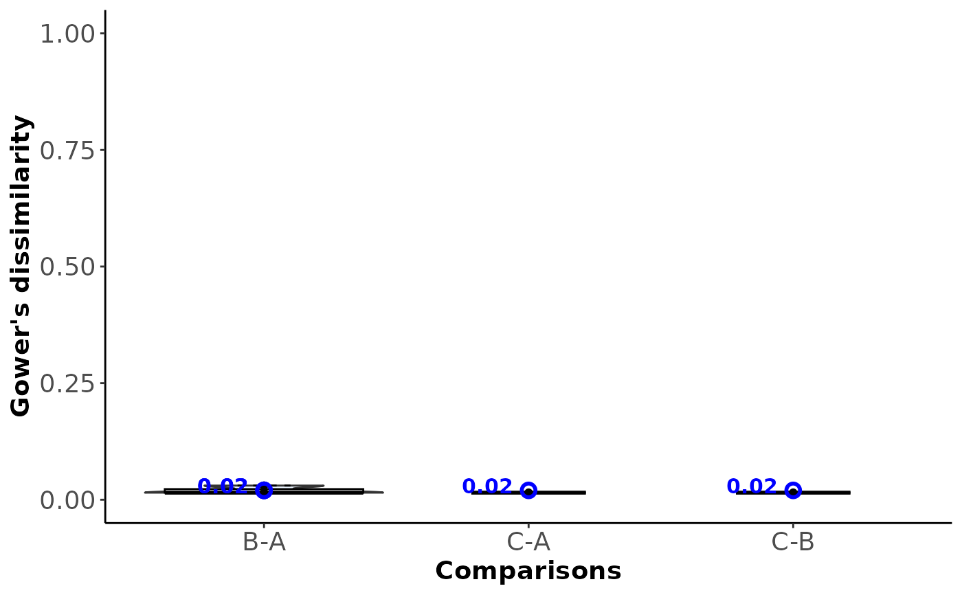
Within_comparison_dissimilarity: A violin plot with integrated box plots and dots on the study dissimilarities per observed comparison (x-axis). Violins are sorted in descending order of the within-comparison dissimilarities (blue point).
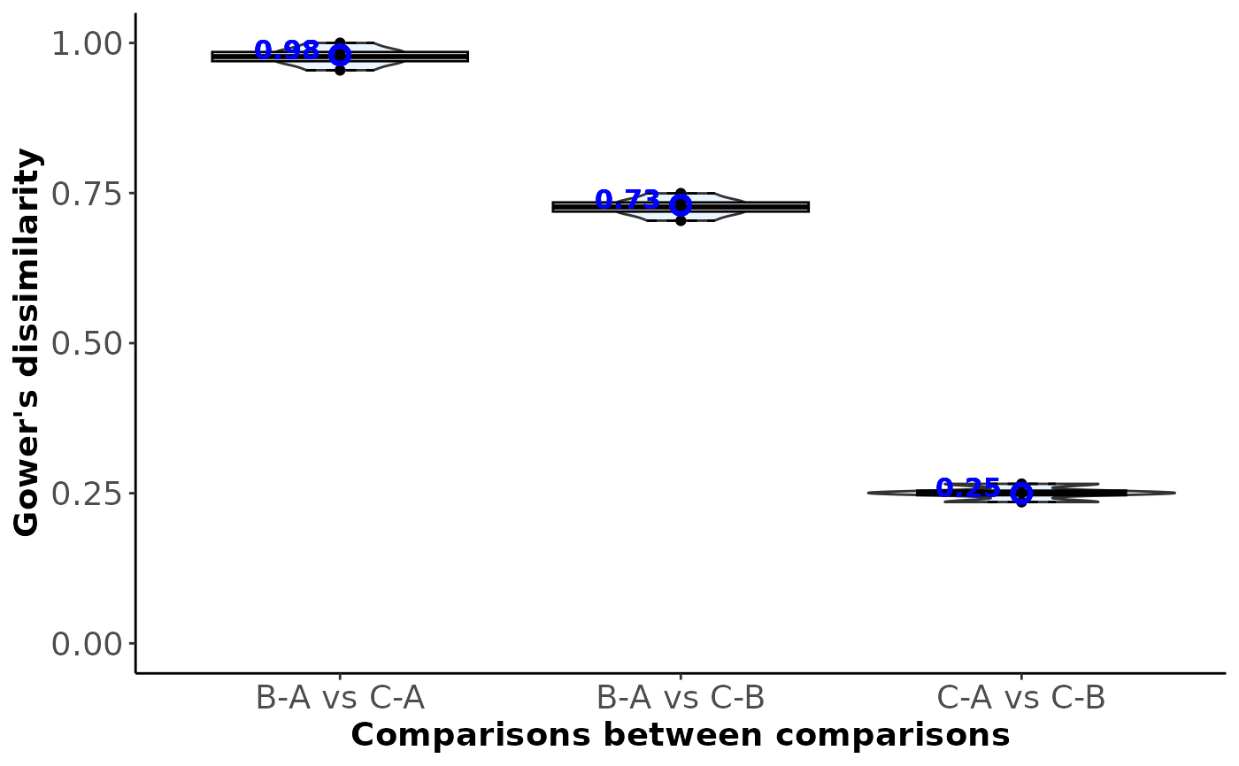
Between_comparison_dissimilarity: A violin plot with integrated box plots and dots on the study dissimilarities per comparison between comparisons (x-axis). Violins are sorted in descending order of the between-comparison dissimilarities (blue point).
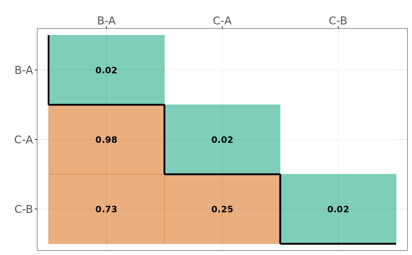
Dissimilarity_heatmap: A heatmap on within-comparison and between-comparison dissimilarities when (informative = TRUE). Diagonal elements refer to within-comparison dissimilarity, and off-diagonal elements refer to between-comparisons dissimilarity. Using a threshold of high similarity (specified using the argument threshold), cells equal or above this threshold are highlighted in orange; otherwise, in green. This heatmap aids in finding 'hot spots' of comparisons that may violate the plausibility of transitivity in the network. Single-study comparisons are indicated with white numbers.
Profile_plot: A profile plot on the average silhouette width for a range of 2 to P-1 clusters, with P being the number of trials. The candidate optimal number of clusters is indicated with a red point directly on the line.
Silhouette_width_plot: A silhouette plot illustrating the silhouette width for each trial, with the trials sorted in decreasing order within the cluster they belong. This output is obtained by calling the silhouette function in the R-package cluster.
Barplot_comparisons_cluster: As stacked barplot on the percentage trials of each comparison found in the clusters (based on the argument optimal_clusters.

Details

The correct type mode of columns in input must be ensured to use the function comp_clustering. The first three columns referring to the trial name, first and second arm of the comparison, respectively, must be character. The remaining columns referring to the characteristics must be double or integer depending on whether the corresponding characteristic refers to a quantitative or qualitative variable. The type mode of each column is assessed by comp_clustering using the base function typeof. Note that comp_clustering invites unordered and ordered variables; for the latter, add the argument ordered = TRUE in the base function factor().

The interventions should be sorted in an ascending order of their identifier number within the trials so that the first intervention column (second column in input) is the control arm for every pairwise comparison. This is important to ensure consistency in the intervention order within the comparisons obtained from the other related functions.

comp_clustering excludes from the dataset the following type of characteristics: (i) completely missing characteristics and (ii) characteristics with missing values in all but one studies for at least one non-single-stufy comparison. Then it proceeds with the clustering process.

The cophenetic correlation coefficient is calculated using the cophenetic function alongside the hclust function for selected linkage methods.

comp_clustering can be used only for a network with at least three comparisons. Otherwise, the execution of the function will be stopped and an error message will be printed on the R console.

References

Gower J. General Coefficient of Similarity and Some of Its Properties. Biometrics 1971;27(4):857–71. doi: 10.2307/2528823

Sokal R, Rohlf F. The Comparison of Dendrograms by Objective Methods. Int Assoc Plant Taxon 1962;11(2):33–40. doi: 10.2307/1217208

Handl J, Knowles J, Kell DB. Computational cluster validation in post-genomic data analysis. Biometrics 2005;21(15):3201–120. doi: 10.1093/bioinformatics/bti517

Rousseeuw PJ. Silhouettes: A graphical aid to the interpretation and validation of cluster analysis. J Comput Appl Math 1987;20:53–65.

Author

Loukia M. Spineli

Examples

# \donttest{
# Fictional dataset
data_set <- data.frame(Trial_name = as.character(1:7),
                      arm1 = c("1", "1", "1", "1", "1", "2", "2"),
                      arm2 = c("2", "2", "2", "3", "3", "3", "3"),
                      sample = c(140, 145, 150, 40, 45, 75, 80),
                      age = c(18, 18, 18, 48, 48, 35, 35),
                      blinding = factor(c("yes", "yes", "yes", "no", "no", "no", "no")))

# Obtain comparison dissimilarities (informative = TRUE)
comp_clustering(input = data_set,
                drug_names = c("A", "B", "C"),
                threshold = 0.13,  # General research setting
                informative = TRUE,
                get_plots = TRUE)
#> - 3 observed comparisons (0 single-study comparisons)
#> - Dropped characteristics: none
#> $Trials_diss_table
#>       1 B-A 2 B-A 3 B-A 4 C-A 5 C-A 6 C-B 7 C-B
#> 1 B-A 0.000    NA    NA    NA    NA    NA    NA
#> 2 B-A 0.015 0.000    NA    NA    NA    NA    NA
#> 3 B-A 0.030 0.015 0.000    NA    NA    NA    NA
#> 4 C-A 0.970 0.985 1.000 0.000    NA    NA    NA
#> 5 C-A 0.955 0.970 0.985 0.015 0.000    NA    NA
#> 6 C-B 0.719 0.734 0.749 0.251 0.235 0.000    NA
#> 7 C-B 0.704 0.719 0.734 0.266 0.251 0.015     0
#> 
#> $Comparisons_diss_table
#>      B-A  C-A  C-B
#> B-A 0.02   NA   NA
#> C-A 0.98 0.02   NA
#> C-B 0.73 0.25 0.02
#> 
#> $Total_dissimilarity
#>   comparison total_dissimilarity         index_type
#> 5 C-A vs C-B                0.25 Between-comparison
#> 3 B-A vs C-B                0.73 Between-comparison
#> 2 B-A vs C-A                0.98 Between-comparison
#> 1        B-A                0.02  Within-comparison
#> 4        C-A                0.02  Within-comparison
#> 6        C-B                0.02  Within-comparison
#> 
#> $Types_used
#>   characteristic    type
#> 1         sample  double
#> 2            age  double
#> 3       blinding integer
#> 
#> $Total_missing
#> [1] "0%"
#> 
#> $Within_comparison_dissimilarity

#> 
#> $Between_comparison_dissimilarity

#> 
#> $Dissimilarity_heatmap

#> 
#> attr(,"class")
#> [1] "comp_clustering"
# }