Dendrogram with amalgamated heatmap (Comparisons' comparability for transitivity evaluation)
Source:R/dendro.heatmap_function.R
dendro_heatmap.Rddendro_heatmap creates a dendrogram alongside the heatmap of
Gower dissimilarities among the trials in the network for a specific
linkage method and number of clusters (Spineli et al., 2025).
Arguments
- input
An object of S3 class
comp_clustering. See 'Value' incomp_clustering.- label_size
A positive integer for the font size of the heatmap elements.
label_sizedetermines the size argument found in the geom's aesthetic properties in the R-package ggplot2.- axis_text_size
A positive integer for the font size of row and column names of the heatmap.
axis_text_sizedetermines the axis.text argument found in the theme's properties in the R-package ggplot2.
Value
dendro_heatmap uses the heatmaply
function of the R-package
heatmaply to create a
cluster heatmap for a selected linkage method and number of clusters. The
function uses different colours to indicate the clusters directly on the
dendrogram, specified using the R-package
dendextend. The names
of the leaves refer to the trials and corresponding pairwise comparison.
@details
The function inherits the linkage method and number of optimal clusters by
the comp_clustering function.
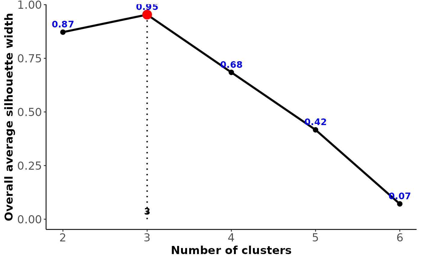
Remember: when using the comp_clustering function, inspect
the average silhouette width for a wide range of clusters to decide on the
optimal number of clusters.
References
Spineli LM, Papadimitropoulou K, Kalyvas C. Exploring the Transitivity Assumption in Network Meta-Analysis: A Novel Approach and Its Implications. Stat Med 2025;44(7):e70068. doi: 10.1002/sim.70068.
Examples
# \donttest{
# Fictional dataset
data_set <- data.frame(Trial_name = as.character(1:7),
arm1 = c("1", "1", "1", "1", "1", "2", "2"),
arm2 = c("2", "2", "2", "3", "3", "3", "3"),
sample = c(140, 145, 150, 40, 45, 75, 80),
age = c(18, 18, 18, 48, 48, 35, 35),
blinding = as.integer(c("yes", "yes", "yes", "no", "no", "no", "no")))
#> Warning: NAs introduced by coercion
# Apply hierarchical clustering (informative = FALSE)
hier <- comp_clustering(input = data_set,
drug_names = c("A", "B", "C"),
threshold = 0.13, # General research setting
informative = FALSE,
optimal_clusters = 3,
get_plots = TRUE)
#> - 3 observed comparisons (0 single-study comparisons)
#> - Dropped characteristics: blinding
#> Warning: data length [63] is not a sub-multiple or multiple of the number of columns [2]
#> - Cophenetic coefficient: 0.911
#> - Optimal linkage method: average
#> $Trials_diss_table
#> 1 B-A 2 B-A 3 B-A 4 C-A 5 C-A 6 C-B 7 C-B
#> 1 B-A 0.000 NA NA NA NA NA NA
#> 2 B-A 0.023 0.000 NA NA NA NA NA
#> 3 B-A 0.045 0.023 0.000 NA NA NA NA
#> 4 C-A 0.955 0.977 1.000 0.000 NA NA NA
#> 5 C-A 0.932 0.955 0.977 0.023 0.000 NA NA
#> 6 C-B 0.579 0.602 0.624 0.376 0.353 0.000 NA
#> 7 C-B 0.556 0.579 0.602 0.398 0.376 0.023 0
#>
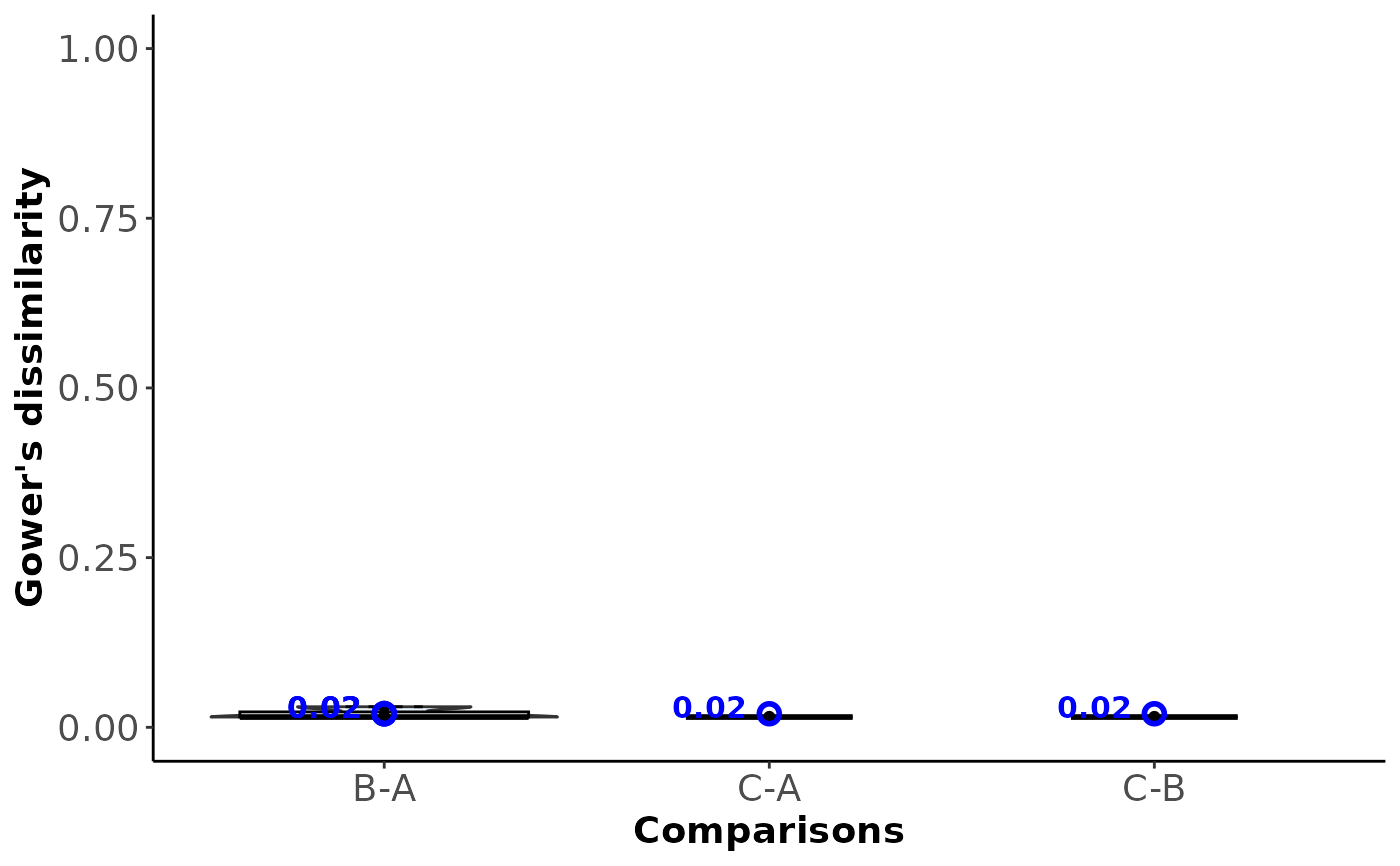
#> $Comparisons_diss_table
#> B-A C-A C-B
#> B-A 0.03 NA NA
#> C-A 0.97 0.02 NA
#> C-B 0.59 0.38 0.02
#>
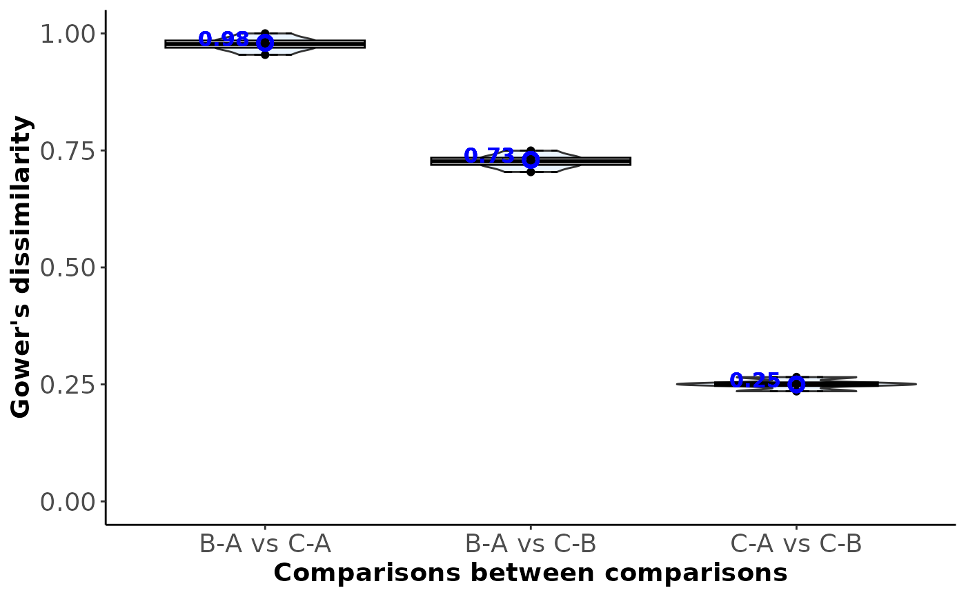
#> $Total_dissimilarity
#> comparison total_dissimilarity index_type
#> 5 C-A vs C-B 0.38 Between-comparison
#> 3 B-A vs C-B 0.59 Between-comparison
#> 2 B-A vs C-A 0.97 Between-comparison
#> 4 C-A 0.02 Within-comparison
#> 6 C-B 0.02 Within-comparison
#> 1 B-A 0.03 Within-comparison
#>
#> $Types_used
#> characteristic type
#> 1 sample double
#> 2 age double
#> 3 blinding integer
#>
#> $Total_missing
#> [1] "33.33%"
#>
#> $Table_average_silhouette_width
#> clusters silhouette
#> 1 2 0.782
#> 2 3 0.943
#> 3 4 0.608
#> 4 5 0.339
#> 5 6 0.071
#>
#> $Table_cophenetic_coefficient
#> linkage_methods results
#> 5 average 0.911
#> 6 mcquitty 0.911
#> 7 median 0.910
#> 8 centroid 0.909
#> 4 complete 0.908
#> 2 ward.D2 0.907
#> 1 ward.D 0.902
#> 3 single 0.901
#>
#> $Optimal_link
#> [1] "average"
#>
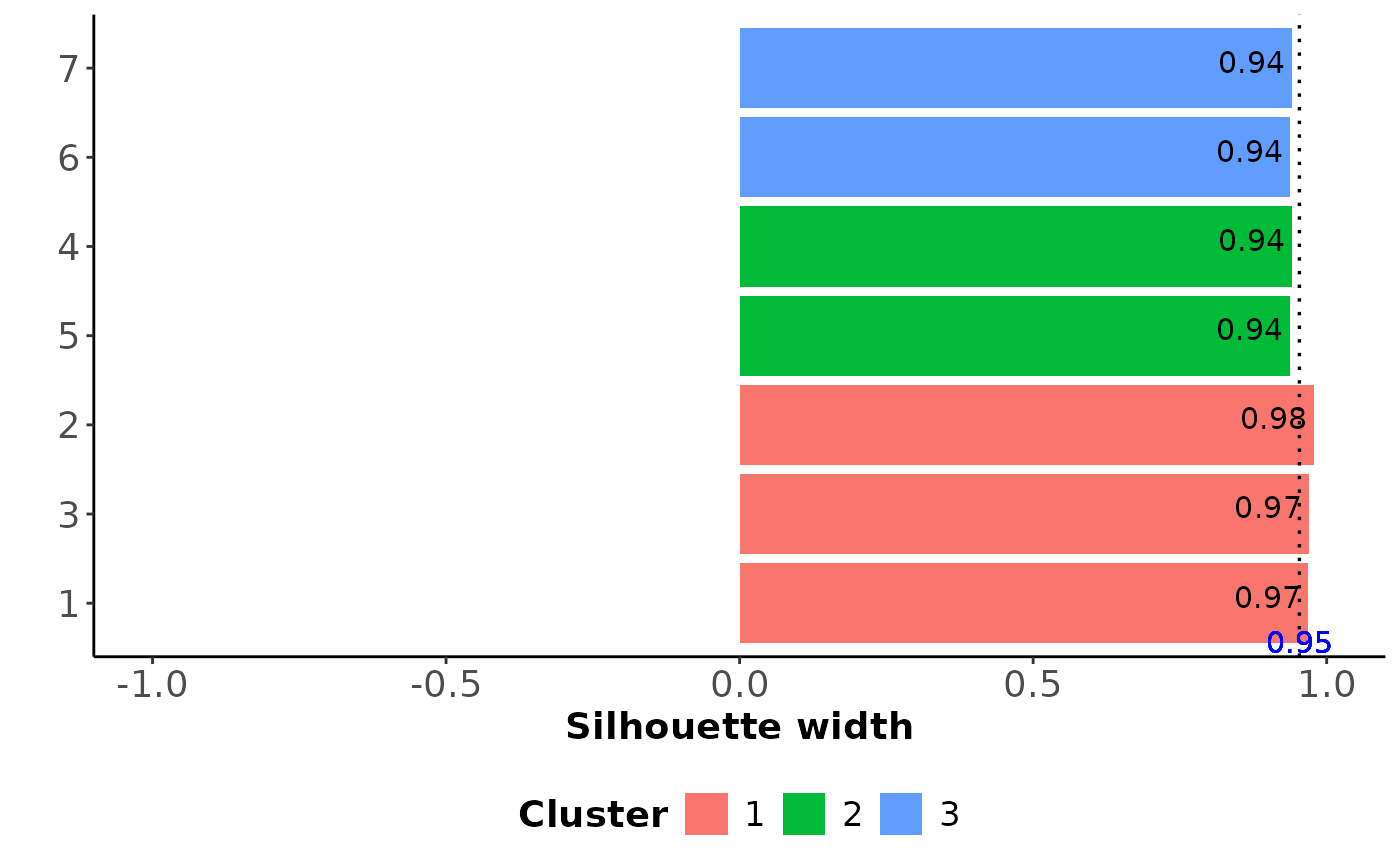
#> $Cluster_comp
#> study cluster sil_width
#> 1 1 1 0.9399199
#> 2 2 1 0.9614891
#> 3 3 1 0.9443758
#> 4 4 2 0.9412916
#> 5 5 2 0.9376299
#> 6 6 3 0.9376299
#> 7 7 3 0.9412916
#>
#> $Within_comparison_dissimilarity
 #>
#> $Between_comparison_dissimilarity
#>
#> $Between_comparison_dissimilarity
 #>
#> $Profile_plot
#>
#> $Profile_plot
 #>
#> $Silhouette_width_plot
#>
#> $Silhouette_width_plot
 #>
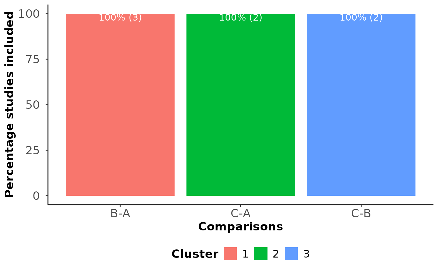
#> $Barplot_comparisons_cluster
#>
#> $Barplot_comparisons_cluster
 #>
#> attr(,"class")
#> [1] "comp_clustering"
# Create the dendrogram with integrated heatmap
dendro_heatmap(hier)
#> Warning: Using `size` aesthetic for lines was deprecated in ggplot2 3.4.0.
#> ℹ Please use `linewidth` instead.
#> ℹ The deprecated feature was likely used in the dendextend package.
#> Please report the issue at <https://github.com/talgalili/dendextend/issues>.
# }
#>
#> attr(,"class")
#> [1] "comp_clustering"
# Create the dendrogram with integrated heatmap
dendro_heatmap(hier)
#> Warning: Using `size` aesthetic for lines was deprecated in ggplot2 3.4.0.
#> ℹ Please use `linewidth` instead.
#> ℹ The deprecated feature was likely used in the dendextend package.
#> Please report the issue at <https://github.com/talgalili/dendextend/issues>.
# }