End-user-ready results for a series of pairwise meta-analyses

Facilitates the comparison of the consistency model (via run_model) with a series of pairwise meta-analyses (via run_series_meta) regarding the estimated summary effect sizes and between-trial standard deviation for comparisons with at least two trials.

Usage

series_meta_plot(full, meta, drug_names, save_xls)

Arguments

full: An object of S3 class run_model. See 'Value' in run_model.
meta: An object of S3 class run_series_meta. See 'Value' in run_series_meta.
drug_names: A vector of labels with the name of the interventions in the order they appear in the argument data of run_model. If drug_names is not defined, the order of the interventions as they appear in data is used, instead.
save_xls: Logical to indicate whether to export the tabulated results to an 'xlsx' file (via the write_xlsx function of the R-package writexl) at the working directory of the user. The default is FALSE (do not export).

Value

The R console prints the data-frame with the estimated summary effect sizes and between-trial standard deviation of comparisons under both models. The comparisons have at least two trials. In the case of a fixed-effect model, the data-frame is printed without the results on the between-trial standard deviation.

Furthermore, series_meta_plot exports the data-frame to an 'xlsx' file at the working directory of the user.

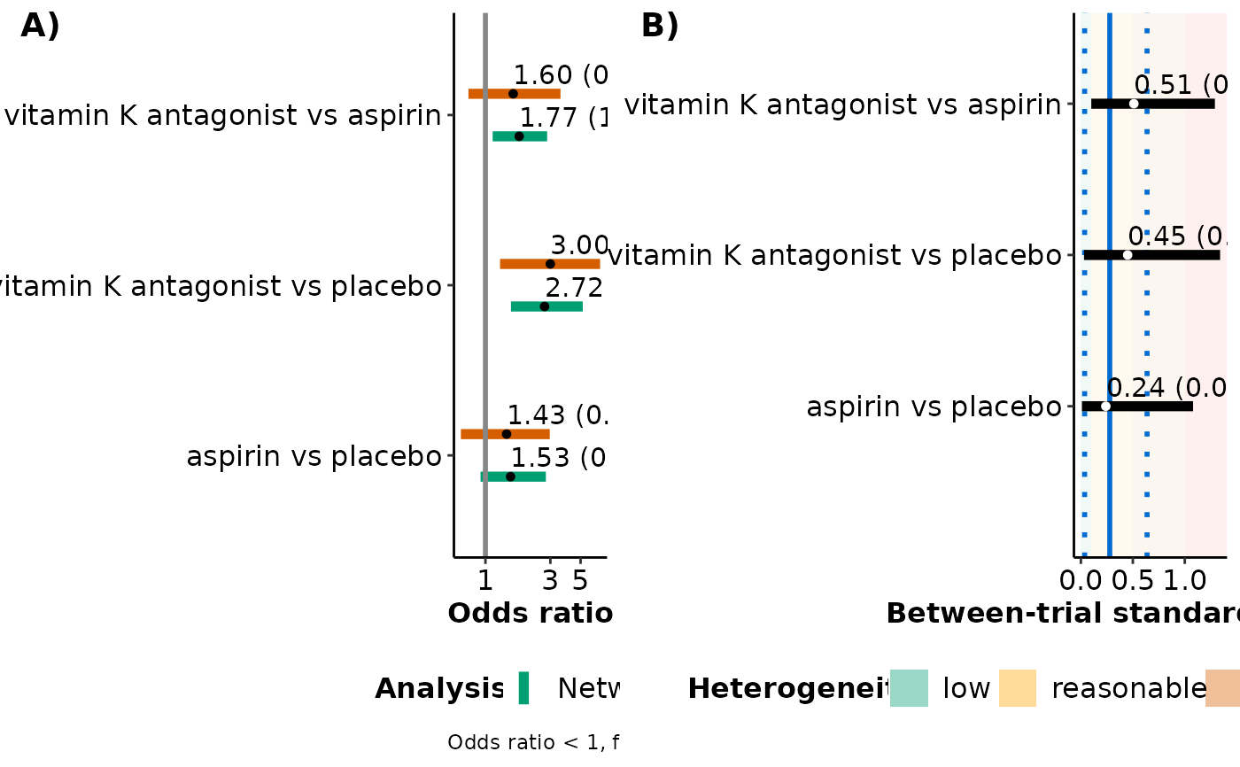
series_meta_plot returns a panel of two forest plots: (1) a forest plot on the posterior median and 95% credible interval of the summary effect size for the observed comparisons from network meta-analysis and the corresponding pairwise meta-analyses, and (2) a forest plot on the posterior median and 95% credible interval of the between-trial standard deviation for these observed comparisons. The estimated median and 95% credible intervals of the between-trial standard deviation from network meta-analysis appear in the forest plot as a solid and two dotted parallel blue lines, respectively. The different levels of heterogeneity appear as green, yellow, orange, and red rectangles to indicate a low, reasonable, fairly high, and fairly extreme heterogeneity, respectively, following the classification of Spiegelhalter et al. (2004). When a fixed-effect model has been fitted, only the forest plot on the estimated summary effect sizes is shown.

Details

series_meta_plot can be used only for a network of interventions. Otherwise, the execution of the function will be stopped and an error message will be printed on the R console.

For a binary outcome, when measure is "RR" (relative risk) or "RD" (risk difference) in run_model, series_meta_plot currently presents the results in the odds ratio for being the base-case effect measure in run_model for a binary outcome (see also 'Details' in run_model).

The user can detect any inconsistencies in the estimated effects from the compared models and explore the gains in precision stemming from applying network meta-analysis. Furthermore, the user can investigate the plausibility of the common between-trial heterogeneity assumption which is typically considered in network meta-analysis.

References

Spiegelhalter DJ, Abrams KR, Myles JP. Bayesian approaches to clinical trials and health-care evaluation. John Wiley and Sons, Chichester, 2004.

Author

Loukia M. Spineli

Examples

data("nma.dogliotti2014")

# Read results from 'run_model' (using the default arguments)
res <- readRDS(system.file('extdata/res_dogliotti.rds', package = 'rnmamod'))

# Read results from 'run_series_meta' (using the default arguments)
meta <- readRDS(system.file('extdata/meta_dogliotti.rds',
                package = 'rnmamod'))

# The names of the interventions in the order they appear in the dataset
interv_names <- c("placebo", "aspirin", "aspirin plus clopidogrel",
                  "dabigatran 110 mg", "dabigatran 150 mg", "rivaroxaban",
                  "vitamin K antagonist", "apixaban")

# Plot the results from both models
series_meta_plot(full = res,
                 meta = meta,
                 drug_names = interv_names)
#> $tabulated_results
#> 
#> 
#> Table: Estimation for each observed comparison
#> 
#> |Comparison                      |Median NMA |SD NMA |95% CrI NMA   |Median MA |SD MA |95% CrI MA    |Median tau |SD tau |95% CrI tau  |
#> |:-------------------------------|:----------|:------|:-------------|:---------|:-----|:-------------|:----------|:------|:------------|
#> |aspirin vs placebo              |1.53       |0.27   |(0.92, 2.78)  |1.43      |0.37  |(0.66, 2.97)  |0.24       |0.28   |(0.01, 1.08) |
#> |vitamin K antagonist vs placebo |2.72       |0.30   |(1.54, 5.19)* |3.00      |0.42  |(1.28, 6.96)* |0.45       |0.34   |(0.03, 1.34) |
#> |vitamin K antagonist vs aspirin |1.77       |0.23   |(1.13, 2.84)* |1.60      |0.39  |(0.75, 3.56)  |0.51       |0.30   |(0.10, 1.29) |
#> 
#> $forest_plots

#>